Why Understanding 802.11 MCS Index Rates Drive Accurate AP Density Planning
MCS is the PHY layer’s truth. If you don’t design backward from it, you’re placing APs by instinct, not physics.
Key Takeaways
- The MCS index encodes modulation order, coding rate, guard interval, and spatial streams, it is the PHY layer’s single source of truth for throughput potential.
- Higher-order QAM (256-QAM, 1024-QAM) requires progressively higher SNR margins. If the link can’t sustain that margin, the client steps down, and the whole BSS pays the airtime tax.
- AP density is SNR engineering, not coverage engineering. Shorter cell radii raise RSSI, reduce TX power, and keep co-channel interference in check.
- CCA is the hidden breaking point. A design that looks clean on a heat map can collapse under real load when too many APs or clients trigger deferred transmissions.
- Start from MCS, work backward: required throughput → required MCS → required SNR → required AP spacing → verify against CCA, noise floor, and management overhead.
Table of Contents
1. The MCS Index: PHY Layer Truth
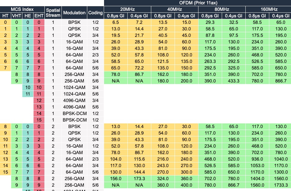
Designing a WLAN that delivers predictable throughput requires understanding how 802.11 clients choose their Modulation and Coding Scheme. The MCS index is the PHY layer’s truth. It reflects modulation order, coding rate, guard interval, and spatial streams. From this index you can infer actual throughput, airtime efficiency, and whether the channel can support the applications you are designing for.
If you want a certain throughput outcome, you need a certain MCS. To get that MCS, you need a certain SNR. To get that SNR, you need the right AP density in the right RF conditions. Everything else is noise.
The MCS table, documented at resources like mcsindex.net, maps each index value to a precise PHY rate (“MCS Index Table”). That rate is the ceiling. What you actually deliver depends on whether the RF environment can sustain the SNR that index requires, and whether contention allows the radio to transmit often enough to reach it.
2. QAM, Coding Rate, and SNR Requirements
Higher MCS values rely on higher-order QAM. BPSK for MCS 0 sits at the bottom. 64-QAM defines the midrange. 256-QAM and 1024-QAM define the high end (Wi-Fi Alliance, “Wi-Fi 6 Technology Introduction”; Wi-Fi Alliance, “Wi-Fi 7 Introduction”). Each jump adds bits per symbol, but the constellation points get closer together. The PHY needs a cleaner signal to decode the symbol without error.
Coding rate influences this further. A rate like 4/5 or 5/6 removes redundancy and increases efficiency. It also tightens SNR requirements because there is less protection against bit errors. Coding at 7/8 or 5/6 requires an SNR buffer that the RF environment must maintain consistently, not just momentarily (IEEE, “IEEE Std 802.11-2020”).
| Modulation | Typical Coding Rate | Approximate SNR Required | Notes |
|---|---|---|---|
BPSK |
1/2 | ~5–10 dB | MCS 0; minimum viable rate; long-range fallback |
QPSK |
1/2 – 3/4 | ~10–15 dB | Reliable at moderate distances |
16-QAM |
1/2 – 3/4 | ~15–20 dB | Mid-range performance |
64-QAM |
2/3 – 5/6 | ~22–28 dB | High-20s dB for 5/6; Wi-Fi 5 top tier |
256-QAM |
3/4 – 5/6 | ~28–32 dB | Wi-Fi 5/6 high tier; ~30 dB required |
1024-QAM |
3/4 – 5/6 | ~33–38 dB | Wi-Fi 6/6E/7; mid-30s or better required |
This produces a strict relationship between SNR and the MCS level the PHY can hold. While exact thresholds vary by chipset, the ranges are well known (Gast, 802.11ac: A Survival Guide; CWNP, “Certified Wireless Network Expert (CWNE) Study Materials”). 64-QAM 5/6 generally needs high-20s dB SNR. 256-QAM often requires around 30 dB. 1024-QAM needs mid-30s or better (Wi-Fi Alliance, “Wi-Fi 7 Introduction”).
If the link cannot supply that margin, the client steps down. Each step down lowers the PHY rate. Lower PHY rates stretch airtime usage because each frame occupies the channel longer, which increases contention. The whole BSS slows, even if only a few clients drop to lower MCS levels.
3. AP Density as SNR Engineering
AP density is the primary tool for shaping the SNR environment. SNR is not just RSSI. It is RSSI minus the composite noise floor. AP density controls RSSI by controlling the maximum distance between the AP and the client. It also influences interference because smaller cells allow you to lower transmit power, which reduces overlap between co-channel APs.
But density is not free. More APs increase beacon traffic, probe response activity, and the number of devices performing clear channel assessments. All of this interacts with MCS stability and capacity. There is a threshold beyond which adding APs actively degrades performance rather than improving it.
Smaller cells raise RSSI. Lower TX power reduces interference between co-channel APs. Both improve SNR. But only if the noise floor cooperates, more on that below.
4. CCA: Where Dense Deployments Break Down
How CCA Works
Clear Channel Assessment (CCA) is a physical layer mechanism that all wireless devices use to determine if the air is busy before transmitting. It is a core component of CSMA/CA, the protocol that prevents multiple devices from transmitting simultaneously on the same channel (IEEE, “IEEE Std 802.11-2020”).
CCA involves two thresholds:
- Energy Detect (ED), triggers when any RF energy rises above a threshold, regardless of modulation
- Preamble Detect (PD), triggers when the radio sees a valid 802.11 preamble above threshold
If energy exceeds ED, or if a preamble is seen above PD, the medium is considered busy. The radio defers and backs off.
CCA in Dense Deployments
Dense deployments cause CCA to fire more often. When too many APs or clients are within ED or PD range, each device senses the medium as busy more frequently, even when the interfering signal is too weak to decode. This effectively stretches contention windows and reduces the airtime available for actual data.
Even with strong RSSI and theoretically sufficient SNR to support a high MCS, a device may not transmit often enough to maintain the associated throughput. CCA can be the breaking point where a design that looks fine on a heat map collapses under real load.
This is why effective AP density is not just a matter of placing more APs. You need enough APs to keep RSSI high and cell sizes controlled, but not so many that CCA turns into a gridlock engine. If the environment is noisy and the ED floor is high, APs will defer more often and lose effective airtime. If RTS/CTS exchanges become frequent due to collisions, airtime efficiency drops further. In that scenario, adding APs does not raise SNR enough to offset the hit from increased contention and CCA activity.
5. Management Traffic and Airtime Budget
Management traffic amplifies the problem. Every AP sends beacons at fixed intervals. Each SSID adds another set of beacons. Clients send probe requests. APs answer with probe responses. Multicast and broadcast traffic transmits at the lowest basic rate, which further expands airtime consumption.
ACK frames, Block ACK frames, RTS/CTS frames, and OBSS-related signaling in Wi-Fi 6 add additional overhead (Wi-Fi Alliance, “Wi-Fi 6 Technology Introduction”). These frames count against the same airtime budget that data frames need to use.
Real throughput ends up at roughly half the PHY rate in the best conditions (Gast, 802.11 Wireless Networks). In congested or poorly designed networks, too many SSIDs, excessive management frames, high noise, usable throughput drops far below half. PHY rate is a ceiling, not a promise.
6. The Noise Floor: The Hard Boundary
The noise floor sets the hard boundary for what is possible. A clean environment with a noise floor around -92 dBm or -95 dBm gives a wide SNR margin (CWNP, “Certified Wireless Network Expert (CWNE) Study Materials”). You can achieve high MCS values with modest RSSI. You can deploy more APs without triggering excessive CCA. You can shrink cells to stabilize MCS.
But if the noise floor rises to -80 dBm or -78 dBm because of external interference, your entire design collapses (CWNP, “Certified Wireless Network Expert (CWNE) Study Materials”). The same RSSI no longer provides enough SNR to hold high-order QAM. CCA triggers earlier. Contention rises.
Adding more APs does not help when the SNR ceiling is physically limited by the environment. If the noise floor is elevated, you cannot engineer your way out of it with density alone. You have to fix the noise source, or accept a lower MCS target.
7. The Design Framework: Working Backward from MCS
A correct design starts with MCS requirements. Work the chain in this order:
# Step 1: Define the throughput requirement per client/application
Required throughput → determines airtime needed

# Step 2: Select the MCS that can deliver that airtime efficiency
Required airtime → select MCS index

# Step 3: Determine the SNR the PHY must sustain for that MCS
MCS index → minimum SNR (e.g., 1024-QAM 5/6 → ~35+ dB)

# Step 4: Determine AP spacing that achieves the required RSSI/SNR
SNR target → maximum AP-to-client distance → AP density

# Step 5: Validate the design against real-world constraints
- Does CCA fire so often that airtime is lost?
- Does the noise floor cap achievable SNR?
- Does management traffic (beacons, probes, ACKs) exhaust airtime budget?
- Does TX power reduction (from tighter cells) reduce co-channel interference?
Only if all these layers align does the design work. This is the difference between placing APs by coverage and designing WLANs by physics.
Once you understand how MCS, SNR, CCA, coding rate, and noise floor interact, AP density becomes a measurable engineering decision instead of guesswork. Every capacity calculation you run traces back to that table.

References
- IEEE. “IEEE Standard for Information Technology–Telecommunications and Information Exchange between Systems – Local and Metropolitan Area Networks–Specific Requirements – Part 11: Wireless LAN Medium Access Control (MAC) and Physical Layer (PHY) Specifications.” IEEE Std 802.11-2020, IEEE, 26 Feb. 2021.
- Wi-Fi Alliance. “Wi-Fi 6 Technology Introduction.” Wi-Fi Alliance White Paper, Wi-Fi Alliance, 2019, http://www.wi-fi.org.
- Wi-Fi Alliance. “Wi-Fi 7 Introduction.” Wi-Fi Alliance White Paper, Wi-Fi Alliance, 2024, http://www.wi-fi.org.
- CWNP. “Certified Wireless Network Expert (CWNE) Study Materials.” CWNP Program, CWNP, 2024, http://www.cwnp.com.
- Gast, Matthew S. 802.11ac: A Survival Guide. O’Reilly Media, 2013.
- Gast, Matthew S. 802.11 Wireless Networks: The Definitive Guide. 2nd ed., O’Reilly Media, 2005.
- “MCS Index Table.” mcsindex.net, mcsindex.net. Accessed 8 Jan. 2025.